Mathematics for AI: Linear Algebra

Scalars, Vectors, Matrices, Tensors

import numpy as np

# Scalars
# Definition: A single number (0D), e.g., a learning rate in AI models
learning_rate = 0.01  # Scalar for gradient descent step size
print("Scalar (Learning Rate):", learning_rate)
# Real-world: Controls how fast a neural network learns
# Operation: Simple arithmetic
scaled_value = learning_rate * 100
print("Scaled Scalar:", scaled_value)

# Vectors
# Definition: 1D array, e.g., feature vector in machine learning
feature_vector = np.array([0.5, 0.8, 0.2])  # Represents a data point (e.g., customer purchase history)
print("\nVector (Feature Vector):", feature_vector)
# Real-world: Used in recommendation systems or word embeddings
# Operation: Dot product (measures similarity)
another_vector = np.array([0.1, 0.4, 0.7])
dot_product = np.dot(feature_vector, another_vector)
print("Dot Product:", dot_product)

# Matrices
# Definition: 2D array, e.g., for image data or linear transformations
image_patch = np.array([[1, 2, 3], [4, 5, 6]])  # 2x3 matrix (e.g., grayscale image patch)
print("\nMatrix (Image Patch):\n", image_patch)
# Real-world: Used in CNNs for image processing
# Operation: Matrix multiplication (e.g., for transformations)
weights = np.array([[0.1, 0.2], [0.3, 0.4], [0.5, 0.6]])  # 3x2 weight matrix
result = np.matmul(image_patch, weights)  # 2x2 result
print("Matrix Multiplication Result:\n", result)

# Tensors
# Definition: nD array (n≥0), e.g., for RGB images or video data
rgb_image = np.random.rand(224, 224, 3)  # 3D tensor (height, width, RGB channels)
print("\nTensor (RGB Image Shape):", rgb_image.shape)
# Real-world: Input to CNNs like ResNet for image classification
# Operation: Tensor slicing (e.g., extract red channel)
red_channel = rgb_image[:, :, 0]  # First channel (R)
print("Red Channel Shape:", red_channel.shape)
# Example: 4D tensor for a batch of images
batch_images = np.random.rand(2, 4, 4, 3)  # Batch of 2 RGB 4x4 images
print("Batch Tensor:", batch_images)

Scalar (Learning Rate): 0.01
Scaled Scalar: 1.0

Vector (Feature Vector): [0.5 0.8 0.2]
Dot Product: 0.51

Matrix (Image Patch):
 [[1 2 3]
 [4 5 6]]
Matrix Multiplication Result:
 [[2.2 2.8]
 [4.9 6.4]]

Tensor (RGB Image Shape): (224, 224, 3)
Red Channel Shape: (224, 224)
Batch Tensor Shape: [[[[0.04087357 0.57134536 0.32519568]
   [0.34167714 0.62335238 0.46628049]
   [0.07720674 0.77133272 0.36870046]
   [0.72117031 0.04701737 0.86162155]]

  [[0.85597285 0.14884848 0.48867849]
   [0.85831712 0.9510796  0.58200469]
   [0.57347744 0.24808471 0.41284116]
   [0.8178081  0.97333519 0.10092528]]

  [[0.04708062 0.04044213 0.22104739]
   [0.08955609 0.82080325 0.11358177]
   [0.91882124 0.60249004 0.72110625]
   [0.12282592 0.6878657  0.75100109]]

  [[0.79111113 0.02168534 0.89053718]
   [0.62379676 0.28582163 0.36874591]
   [0.29939015 0.49078382 0.96479222]
   [0.9737543  0.02131901 0.03780112]]]


 [[[0.89632584 0.97437265 0.16876449]
   [0.64941646 0.63884824 0.98995114]
   [0.44964252 0.72292501 0.44936663]
   [0.7425726  0.38513847 0.28983086]]

  [[0.31092603 0.88805527 0.1764936 ]
   [0.16567742 0.49115005 0.49396291]
   [0.01596826 0.98731473 0.70769769]
   [0.25895077 0.37736448 0.73386227]]

  [[0.09645565 0.36557884 0.39174251]
   [0.79035446 0.33778424 0.47940533]
   [0.64473504 0.038141   0.17750133]
   [0.78799436 0.35127631 0.31383826]]

  [[0.02208777 0.60393952 0.44482964]
   [0.29335764 0.16871938 0.34279193]
   [0.9368042  0.80870572 0.74452877]
   [0.67187876 0.11662868 0.86089061]]]]

Scalars

• Definition/Explanation: A scalar is a single numerical value, representing magnitude without direction.
  • Scalars can be integers, floating-point numbers, or complex numbers.
  • Used in operations like scaling vectors or adjusting model parameters.
  • Typically denoted by lowercase letters (e.g., (a), (b)).

In AI, scalars are used to represent constants, weights, or scaling factors.

• Examples:
  • Learning rate in gradient descent (( $\alpha = 0.01$ )).
  • A pixel intensity value in an image (e.g., 255 for white in grayscale).
• Why It Matters:
  • Scalars are fundamental in AI for parameter tuning (e.g., learning rates in neural networks).
  • Real-world: Adjusting the learning rate in a neural network to optimize training speed and accuracy.

---

Vectors

• Definition/Explanation: A vector is an ordered list of scalars, representing magnitude and direction in a multidimensional space.
  • Represented as 1D arrays (e.g., ( $\mathbf{v} = [v_1, v_2, \dots, v_n]$ )).
  • Operations: addition, dot product, scaling.
  • Used in feature representation and embeddings.

In AI, vectors represent data points, features, or weights.

• Examples:
  • A feature vector for a house: $[1200, 3, 2]$ (square footage, bedrooms, bathrooms).
  • Word embeddings in NLP (e.g., Word2Vec output: $[0.5, -0.2, 0.1, \dots]$).
• Why It Matters:
  • Vectors are core to machine learning, representing data in models like SVMs or neural networks.
  • Real-world: Encoding user preferences in recommendation systems (e.g., Netflix movie preferences as a vector).

---

Matrices

• Definition/Explanation: A matrix is a 2D array of scalars, organized in rows and columns.
  • Denoted as $A \in \mathbb{R}^{m \times n}$ ($m$ rows, $n$ columns).
  • Operations: matrix multiplication, transposition, inversion.
  • Used in data storage, transformations, and neural network layers.

 used to represent linear transformations or datasets in AI.

• Examples:
  • A dataset matrix: rows as samples, columns as features (e.g., $1000 \times 5$ for 1000 houses with 5 features).
  • Weight matrix in a neural network layer: $W \in \mathbb{R}^{n \times m}$ connecting input to output neurons.
• Why It Matters:
  • Matrices enable efficient computation in AI, especially in deep learning (e.g., matrix multiplication in GPUs).
  • Real-world: Image processing (e.g., a grayscale image as a matrix of pixel intensities).

++++++++++++++++++++++++++++++++++++++++++++++++++++++++++++++++++++++++++++++++++++++++++++++++++++++++++++++ ++++++++++++++++++++++++++++++++++++++++++++++++++++++++++++++++++++++++++++++++++++++++++++++++++++++++++++++

---

---

Matrix Basics

• Matrix: A rectangular array of numbers. Example:

  $$ A = \begin{bmatrix} 1 & 2 \\ 3 & 4 \end{bmatrix} \in \mathbb{R}^{2 \times 2} $$

• Dimensions: Rows × Columns

---

Matrix Operations

• Addition/Subtraction: Element-wise (same dimensions)

• Scalar Multiplication:

  $$ \alpha A = \begin{bmatrix} \alpha a_{11} & \alpha a_{12} \\ \alpha a_{21} & \alpha a_{22} \end{bmatrix} $$

• Matrix Multiplication:

  $$ C = A \cdot B \quad \text{(valid only if columns of A = rows of B)} $$

• Transpose:

  $$ A^T = \text{flip rows and columns} $$

• Identity Matrix:

  $$ I_n = \text{square matrix with 1s on diagonal} $$

---

Special Matrices

Type	Property Example
Square	Same number of rows and columns
Diagonal	Non-zero entries only on diagonal
Symmetric	$A = A^T$
Orthogonal	$A^T A = I$ (columns are orthonormal)
Zero Matrix	All elements are zero

---

Matrix Inverse

• For $A \in \mathbb{R}^{n \times n}$, $A^{-1}$ satisfies:

  $$ A A^{-1} = A^{-1} A = I $$

• Only exists if $\det(A) \neq 0$ and $A$ is square.

---

Determinant

• Scalar value that can be computed from a square matrix:

  $$ \text{det}(A) $$

• Used to check invertibility and volume scaling.

---

Rank

• Number of linearly independent rows/columns.
• Indicates the dimension of the column space.

---

Trace

• Sum of diagonal elements of a square matrix:

  $$ \text{tr}(A) = \sum_i a_{ii} $$

---

Eigenvalues and Eigenvectors

• For $A \vec{v} = \lambda \vec{v}$:

  • $\lambda$: eigenvalue
  • $\vec{v}$: eigenvector

---

Matrix Decompositions

Type	Form	Use Case
LU	$A = LU$	Solving systems
QR	$A = QR$	Least squares, orthogonal bases
SVD	$A = U \Sigma V^T$	PCA, compression, LSA
Eigendecomp	$A = V \Lambda V^{-1}$	PCA, diagonalization

---

Applications in ML/AI

Matrix Concept	Application
Multiplication	Neural networks, transformations
Transpose	Covariance, dot product
Inverse	Solving linear systems
Rank	Dimensionality and redundancy
SVD/PCA	Dimensionality reduction

---

Matrix Norms & Condition Number

What is a Matrix Norm?

A matrix norm measures the "size", "length", or "magnitude" of a matrix — similar to how a vector norm measures a vector’s length.

Think of it as: “How much can this matrix stretch or shrink a vector?”

---

Common Types of Matrix Norms

Norm	Definition	Interpretation	Example/Notes
Frobenius Norm $|A|_F$	$\sqrt{ \sum_{i,j} a_{ij}^2 }$	Like Euclidean norm for matrices	Used a lot in ML
1-Norm $|A|_1$	Max absolute column sum	Worst-case vertical stretching	$\max_j \sum_i	a_{ij}	$
Infinity Norm $|A|_\infty$	Max absolute row sum	Worst-case horizontal stretching	$\max_i \sum_j	a_{ij}	$
2-Norm (Spectral Norm) $|A|_2$	Largest singular value of $A$	Max stretching factor along any direction	Related to principal component, SVD, etc.

---

Example (Frobenius Norm):

$$ A = \begin{bmatrix} 1 & 2 \\ 3 & 4 \end{bmatrix} \Rightarrow \|A\|_F = \sqrt{1^2 + 2^2 + 3^2 + 4^2} = \sqrt{30} $$

---

---

Condition Number

The condition number tells you how sensitive a system or a matrix operation is to small changes in input.

In ML and numerical algorithms, lower condition numbers = more stable, reliable results.

---

Definition

For a non-singular matrix $A$:

$$ \text{cond}(A) = \|A\| \cdot \|A^{-1}\| $$

• You can use any norm (commonly 2-norm or Frobenius).
• If $\text{cond}(A) \approx 1$: Very stable system
• If $\text{cond}(A) \gg 1$: Unstable or ill-conditioned

---

In terms of singular values:

For 2-norm:

$$ \text{cond}_2(A) = \frac{\sigma_{\text{max}}}{\sigma_{\text{min}}} $$

Where $\sigma$ = singular values from SVD.

---

⚠️ Why It Matters in ML?

Use Case	Impact
Solving Linear Systems	High condition number → errors get amplified
Inverting Matrices	Poor conditioning → instability
Gradient Descent	Ill-conditioned Hessian → slow convergence
Deep Learning	Can cause vanishing/exploding gradients

---

++++++++++++++++++++++++++++++++++++++++++++++++++++++++++++++++++++++++++++++++++++++++++++++++++++++++++++++ ++++++++++++++++++++++++++++++++++++++++++++++++++++++++++++++++++++++++++++++++++++++++++++++++++++++++++++++

---

Moore-Penrose Pseudoinverse

What is the Moore-Penrose Pseudoinverse?

When a matrix doesn’t have an inverse (like when it’s non-square or rank-deficient), we use the pseudoinverse instead.

The Moore-Penrose Pseudoinverse $A^+$ of a matrix $A$ is a generalization of the inverse:

• It works for any matrix (square, rectangular, full-rank, or not).
• It’s the best possible approximate inverse.

---

Denoted by:

$$ A^+ \quad \text{(read: A pseudo-inverse)} $$

If $A$ is a $m \times n$ matrix, then $A^+$ is a $n \times m$ matrix.

---

When Do We Use It?

Scenario	Why use Pseudoinverse
$A$ is not square	So no usual inverse exists
$A$ is not full-rank	Singular matrix (can’t invert)
You want a least-squares solution to $Ax = b$	Regression, ML, Optimization

---

Mathematical Formulation

If $A$ is an $m \times n$ matrix:

• The pseudoinverse $A^+$ is the unique matrix that satisfies:

$$ \begin{aligned} 1. & \quad A A^+ A = A \\ 2. & \quad A^+ A A^+ = A^+ \\ 3. & \quad (A A^+)^T = A A^+ \\ 4. & \quad (A^+ A)^T = A^+ A \end{aligned} $$

---

Computation Using SVD (ML Use Case)

Let:

$$ A = U \Sigma V^T $$

Then the pseudoinverse is:

$$ A^+ = V \Sigma^+ U^T $$

Where $\Sigma^+$ is obtained by:

• Taking reciprocal of each non-zero singular value
• Transposing the diagonal matrix
• Filling remaining entries with zero

---

Least-Squares Solution (ML Use Case)

In ML, we often solve:

$$ Ax = b \quad \text{(no exact solution if overdetermined)} $$

Then the least-squares solution is:

$$ x = A^+ b $$

Used in Linear Regression when $X$ is not square or full-rank.

---

Real ML Applications

Use Case	Why it helps
Linear Regression	$\theta = (X^T X)^{-1} X^T y$ becomes $\theta = X^+ y$ when $X$ isn’t full-rank
Dimensionality Reduction	In SVD, pseudoinverse helps in low-rank approximations
Deep Learning	Used in layer inversion, autoencoders, or backprop through linear layers
Control Systems	Solve under/overdetermined linear systems

---

Pro Tip:

If you're designing ML algorithms from scratch (like in research), or dealing with data where features >> samples (underdetermined), pseudoinverse gives you stable, analytical solutions — no need for iterative solvers.

---

++++++++++++++++++++++++++++++++++++++++++++++++++++++++++++++++++++++++++++++++++++++++++++++++++++++++++++++ ++++++++++++++++++++++++++++++++++++++++++++++++++++++++++++++++++++++++++++++++++++++++++++++++++++++++++++++

---

Kronecker Product & Hadamard Product

What is the Kronecker Product?

The Kronecker product is an operation on two matrices that produces a block matrix. It’s not element-wise, and it’s not the dot product.

For matrices $A \in \mathbb{R}^{m \times n}$ and $B \in \mathbb{R}^{p \times q}$, their Kronecker product $A \otimes B$ is of size $(mp \times nq)$

---

Notation

$$ A \otimes B \quad \text{(pronounced “A kronecker B”)} $$

---

How It Works — Example

Let:

$$ A = \begin{bmatrix} a & b \\ c & d \end{bmatrix}, \quad B = \begin{bmatrix} x & y \\ z & w \end{bmatrix} $$

Then:

$$ A \otimes B = \begin{bmatrix} aB & bB \\ cB & dB \end{bmatrix} = \begin{bmatrix} a x & a y & b x & b y \\ a z & a w & b z & b w \\ c x & c y & d x & d y \\ c z & c w & d z & d w \\ \end{bmatrix} $$

---

---

---

What is the Hadamard Product?

The Hadamard product is an element-wise multiplication between two matrices (or vectors) of the same shape.

If $A, B \in \mathbb{R}^{m \times n}$, then:

$$ A \circ B = [a_{ij} \cdot b_{ij}] $$

🔁 Every element in position $(i, j)$ of the result is the product of $a_{ij} \cdot b_{ij}$.

---

Notation

• $A \circ B$ — Hadamard product
• Sometimes written as A * B (in NumPy, PyTorch, TensorFlow when using element-wise ops)

---

Example

Let:

$$ A = \begin{bmatrix} 1 & 2 \\ 3 & 4 \end{bmatrix}, \quad B = \begin{bmatrix} 5 & 6 \\ 7 & 8 \end{bmatrix} $$

Then:

$$ A \circ B = \begin{bmatrix} 1 \cdot 5 & 2 \cdot 6 \\ 3 \cdot 7 & 4 \cdot 8 \end{bmatrix} = \begin{bmatrix} 5 & 12 \\ 21 & 32 \end{bmatrix} $$

---

Applications in ML & Deep Learning

Use Case	Use
Element-wise operations in ML (e.g., attention, masking)	✅ Hadamard
Creating structured large matrices from small ones	✅ Kronecker
Efficient parameter sharing in deep learning (e.g., tensor compression)	✅ Kronecker

---

Recap

• Dot Product: Projects one vector onto another (returns scalar)
• Outer Product: Expands two vectors to one matrix
• Kronecker Product: expands to a block matrix
• Matrix Multiplication - Follows linear transformation rules
• Hadamard Product - Element-wise multiplication, Combines features/gradients/masks

---

Tensors

• Definition/Explanation: A tensor is a generalized array with arbitrary dimensions, extending scalars (0D), vectors (1D), and matrices (2D) to higher dimensions.

  • Rank: Number of dimensions (e.g., scalar = rank-0, vector = rank-1, matrix = rank-2).
  • Used in deep learning frameworks (e.g., TensorFlow, PyTorch).
  • Operations: tensor contraction, reshaping, slicing.

In AI, tensors store complex data like images or videos.

• Examples:

  • A color image: $256 \times 256 \times 3$ tensor (height, width, RGB channels).
  • A batch of videos: $32 \times 10 \times 720 \times 1280 \times 3$ (batch size, frames, height, width, channels).

• Why It Matters:

  • Tensors handle multidimensional data in deep learning (e.g., CNNs for image recognition).
  • Real-world: Processing 3D medical scans (e.g., MRI images) or video analysis for autonomous driving.

---

Vector Spaces and Subspaces

Vectors

• Definition: An ordered array of numbers (elements), e.g.

  $$ \vec{v} = \begin{bmatrix} 2 \\ -1 \\ 3 \end{bmatrix} \in \mathbb{R}^3 $$

• Operations:

  • Addition: $\vec{a} + \vec{b}$
  • Scalar multiplication: $\alpha \vec{v}$
  • Dot product: $\vec{a} \cdot \vec{b} = \sum a_i b_i$ (produces scalar)

  • Norm (length):

    $$ \|\vec{v}\| = \sqrt{v_1^2 + v_2^2 + \dots + v_n^2} $$

---

Vector Space (Linear Space)

A vector space is a set of vectors that can be added together and multiplied by scalars, and still remain in the set.

Formal Requirements (8 Axioms):

Let $V$ be a vector space over a field $F$ (like ℝ or ℂ). For all $\vec{u}, \vec{v}, \vec{w} \in V$, and $a, b \in F$, the following must hold:

1. Closure under addition: $\vec{u} + \vec{v} \in V$
2. Closure under scalar multiplication: $a\vec{v} \in V$
3. Associativity of addition
4. Commutativity of addition
5. Additive identity: There exists $\vec{0} \in V$ such that $\vec{v} + \vec{0} = \vec{v}$
6. Additive inverse: For every $\vec{v}$, $-\vec{v} \in V$
7. Multiplicative identity: $1\vec{v} = \vec{v}$
8. Distributivity of scalar multiplication over vector addition and over scalar addition

---

Examples of Vector Spaces

Space	Description
$\mathbb{R}^n$	n-dimensional real vectors
Matrices	All $m \times n$ real matrices
Polynomials	Polynomials of degree ≤ n
Functions	All continuous real functions

---

Subspace

A subspace is a subset of a vector space that is also a vector space under the same operations.

Requirements:

For $W \subseteq V$, $W$ is a subspace if:

1. $\vec{0} \in W$ (zero vector included)
2. Closed under vector addition: $\vec{u} + \vec{v} \in W$
3. Closed under scalar multiplication: $c\vec{v} \in W$

Example:

• In $\mathbb{R}^3$, the set of all vectors on the x-y plane (i.e., vectors of form $[x, y, 0]$) is a subspace.

---

Real World ML/AI Examples

1. Word Embeddings & NLP (Natural Language Processing)

   • Vector Space: Words are converted into vectors in a high-dimensional vector space (like 300 dimensions in Word2Vec or 768 in BERT).

   • Why vector spaces? Each word is a point (vector) in this space. Words with similar meanings cluster close to each other — that’s the geometry of meaning.

   • Subspace idea: When you focus on specific topics (say sports-related words), you’re essentially looking at a subspace of the whole embedding space.

   • Real-world: Chatbots, search engines, language translation — all use vector spaces to understand semantic similarity and context.

---

1. Face Recognition Systems

   • What happens? Images of faces are converted into vectors (e.g., using deep learning embeddings).

   • Subspace models: Techniques like Eigenfaces represent face images as points in a face subspace. Recognition happens by comparing projections in this subspace.

---

Why This Matters for You:

Understanding vector spaces and subspaces means you can:

• Build better feature representations.
• Understand how data can be compressed and interpreted.
• Improve model explainability by identifying key directions (basis vectors) in data.
• Innovate by manipulating embeddings and latent spaces.

---

Span & Linear Combination

A linear combination is an expression of the form:

$$ a_1\vec{v}_1 + a_2\vec{v}_2 + \dots + a_n\vec{v}_n $$

Where $a_i$ are scalars and $\vec{v}_i$ are vectors.

---

The span of a set of vectors is all possible linear combinations of those vectors.

$$ \text{Span}(\{\vec{v}_1, \vec{v}_2\}) = \{a_1\vec{v}_1 + a_2\vec{v}_2 \mid a_1, a_2 \in \mathbb{R} \} $$

• Span is always a subspace.

• Example:

  $$ \text{span}\left\{ \begin{bmatrix} 1 \\ 0 \end{bmatrix}, \begin{bmatrix} 0 \\ 1 \end{bmatrix} \right\} = \mathbb{R}^2 $$

• If you span multiple vectors in $\mathbb{R}^n$, the result is a subspace of $\mathbb{R}^n$.

---

Linear Independence

A set of vectors is linearly independent if no vector in the set can be written as a linear combination of the others.

Mathematically:

$$ a_1\vec{v}_1 + a_2\vec{v}_2 + \dots + a_n\vec{v}_n = \vec{0} \Rightarrow a_1 = a_2 = \dots = a_n = 0 $$

• If not, the vectors are linearly dependent.

---

Basis

A basis of a vector space is a set of linearly independent vectors that span the entire space.

• Every vector in the space can be uniquely represented as a linear combination of basis vectors.

Example:

• Standard basis of $\mathbb{R}^2$:

$$ \left\{ \begin{bmatrix} 1 \\ 0 \end{bmatrix}, \begin{bmatrix} 0 \\ 1 \end{bmatrix} \right\} $$

---

Dimension

• The dimension of a vector space is the number of vectors in a basis for that space.
• For $\mathbb{R}^n$, dimension = $n$

---

Projection of a Vector

• Projection of $\vec{a}$ onto $\vec{b}$:

  $$ \text{proj}_{\vec{b}} \vec{a} = \frac{\vec{a} \cdot \vec{b}}{\|\vec{b}\|^2} \vec{b} $$

---

Eigenvalues and Eigenvectors

What are Eigenvalues and Eigenvectors?

• For a square matrix $A \in \mathbb{R}^{n \times n}$, a non-zero vector $\vec{v}$ is an eigenvector if:

$$ A\vec{v} = \lambda \vec{v} $$

• $\lambda$ is the eigenvalue corresponding to eigenvector $\vec{v}$

---

How to Compute

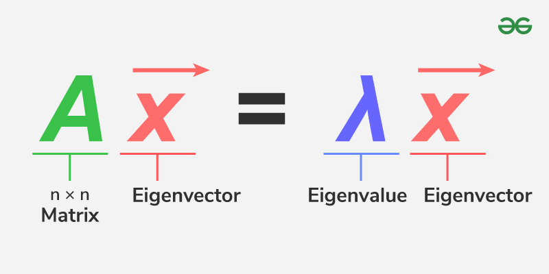
1. Find eigenvalues by solving the characteristic equation:

   $$ \det(A - \lambda I) = 0 $$

2. Find eigenvectors for each $\lambda$ by solving:

   $$ (A - \lambda I)\vec{v} = 0 $$

---

Example

$$ A = \begin{bmatrix} 4 & 1 \\ 2 & 3 \end{bmatrix} $$

• Find eigenvalues by solving:

$$ \det\begin{bmatrix} 4-\lambda & 1 \\ 2 & 3-\lambda \end{bmatrix} = 0 $$$$ (4-\lambda)(3-\lambda) - 2 \times 1 = 0 $$$$ \lambda^2 - 7\lambda + 10 = 0 $$$$ (\lambda - 5)(\lambda - 2) = 0 $$

So eigenvalues: $\lambda_1 = 5, \lambda_2 = 2$

• For $\lambda = 5$, solve $(A - 5I)\mathbf{v} = 0$:

$$ \begin{bmatrix} -1 & 1 \\ 2 & -2 \end{bmatrix} \mathbf{v} = 0 $$

Eigenvector $\mathbf{v}_1 = \begin{bmatrix} 1 \\ 1 \end{bmatrix}$ (up to scalar multiples)

---

Intuitions & Properties

• Intuitions:
  • Applying $A$ to $\mathbf{v}$ only stretches/compresses it, but does not change its direction.
  • Eigenvectors show the “principal directions” of transformation by $A$.
  • Eigenvalues tell how much $\mathbf{v}$ is stretched (if $|\lambda| > 1$) or shrunk (if $|\lambda| < 1$).

• Properties:

  • Eigenvectors corresponding to different eigenvalues are linearly independent.
  • Sum of eigenvalues = trace of matrix $A$ (sum of diagonal entries). $$\text{tr}(A) = \sum \lambda_i$$
  • Product of eigenvalues = determinant of matrix $A$. $$\det(A) = \prod \lambda_i$$
  • If $A$ is symmetric, eigenvalues are real and eigenvectors are orthogonal.

---

Use Cases of Eigenvalues & Eigenvectors

Principal Component Analysis (PCA)

• Purpose: Dimensionality reduction — simplifying complex data while preserving its most important features.
• How: Find eigenvectors of the covariance matrix of data. These eigenvectors (principal components) show directions of maximum variance.
• Benefit: Reduces features, speeds up learning, reduces noise, improves visualization.
• Example: Face recognition, image compression.

Applications in ML/AI

Concept	Application
PCA (Principal Component Analysis)	Find directions (eigenvectors) of max variance
Spectral clustering	Eigenvectors of graph Laplacian for clustering
Stability analysis	Eigenvalues determine system behavior
Markov chains	Eigenvalues define steady states
Neural Networks	Eigenvalues relate to Hessian matrix in optimization

---

Diagonalization

If $A$ has $n$ linearly independent eigenvectors:

$$ A = V \Lambda V^{-1} $$

• $V$: matrix of eigenvectors
• $\Lambda$: diagonal matrix of eigenvalues

---

Spectral Theorem

What Is the Spectral Theorem?

The Spectral Theorem states that any real symmetric matrix can be diagonalized by an orthogonal matrix.

Formally:

If $A \in \mathbb{R}^{n \times n}$ is real symmetric (i.e., $A^T = A$), then:

$$ A = Q \Lambda Q^T $$

Where:

• $Q$ is an orthogonal matrix (columns are orthonormal eigenvectors),
• $\Lambda$ is a diagonal matrix (eigenvalues of $A$).

Intuition

Imagine a real symmetric matrix as a "nice" transformation — like stretching or compressing along specific axes. The Spectral Theorem tells us:

There exists a special coordinate system (formed by the eigenvectors) in which the matrix just scales (not rotates or shears).

---

Linear Transformations

What Is a Linear Transformation?

A linear transformation is a function $T: \mathbb{R}^n \to \mathbb{R}^m$ that satisfies two key properties:

1. Additivity:

   $$ T(\vec{u} + \vec{v}) = T(\vec{u}) + T(\vec{v}) $$

2. Homogeneity (scalar multiplication):

   $$ T(c\vec{v}) = cT(\vec{v}) $$

A transformation is linear if and only if it preserves vector addition and scalar multiplication.

---

Matrix Representation of a Linear Transformation

Every linear transformation can be represented as matrix multiplication:

$$ T(\vec{x}) = A \vec{x} $$

• $A \in \mathbb{R}^{m \times n}$ is the transformation matrix.
• $\vec{x} \in \mathbb{R}^n$ is the input vector.

---

Common Examples of Linear Transformations

Transformation	Matrix $A$	Effect
Identity	$I = \begin{bmatrix} 1 & 0 \\ 0 & 1 \end{bmatrix}$	Leaves vector unchanged
Scaling	$\begin{bmatrix} s & 0 \\ 0 & s \end{bmatrix}$	Enlarges or shrinks vectors
Rotation (2D)	$\begin{bmatrix} \cos\theta & -\sin\theta \\ \sin\theta & \cos\theta \end{bmatrix}$	Rotates vector by $\theta$
Reflection (about x)	$\begin{bmatrix} 1 & 0 \\ 0 & -1 \end{bmatrix}$	Flips over x-axis
Projection onto x-axis	$\begin{bmatrix} 1 & 0 \\ 0 & 0 \end{bmatrix}$	Projects onto horizontal line

---

Kernel and Image

• Kernel (null space): Set of vectors that map to the zero vector:

  $$ \ker(T) = \{ \vec{x} : T(\vec{x}) = \vec{0} \} $$

• Image (range): All vectors that are outputs of $T$:

  $$ \text{Im}(T) = \{ T(\vec{x}) : \vec{x} \in \mathbb{R}^n \} $$

---

Properties of Linear Transformations

Property	Meaning
Linearity	Preserves addition and scalar multiplication
Composable	$T_1(T_2(\vec{x})) = (T_1 \circ T_2)(\vec{x})$
Invertible	Exists $T^{-1}$ such that $T^{-1}(T(\vec{x})) = \vec{x}$
Determined by action on basis	Knowing $T(\vec{e}_i)$ is enough to define $T$

---

Property	Holds If...
One-to-One	$\text{ker}(A) = \{\mathbf{0}\}$
Onto	Columns of $A$ span $\mathbb{R}^m$
Invertible	$A$ is square and full-rank (no zero eigenvalues)

---

Application in ML and Dimensionality Reduction

Use Case	Description
PCA	Projects data to directions of max variance
Feature transformation	Linear mappings in neural networks
Projections	Reduce dimensions while preserving structure
Affine transformations	Linear + translation used in computer vision

---

Affine vs. Linear

• Linear: $T(\vec{x}) = A\vec{x}$
• Affine: $T(\vec{x}) = A\vec{x} + \vec{b}$ (not strictly linear because it doesn't preserve the origin)

---

Inner Product Spaces

What Is an Inner Product Space?

Inner Product (Dot Product in $\mathbb{R}^n$)

For real vectors $\vec{u}, \vec{v} \in \mathbb{R}^n$:

$$ \langle \vec{u}, \vec{v} \rangle = \sum_{i=1}^{n} u_i v_i $$

---

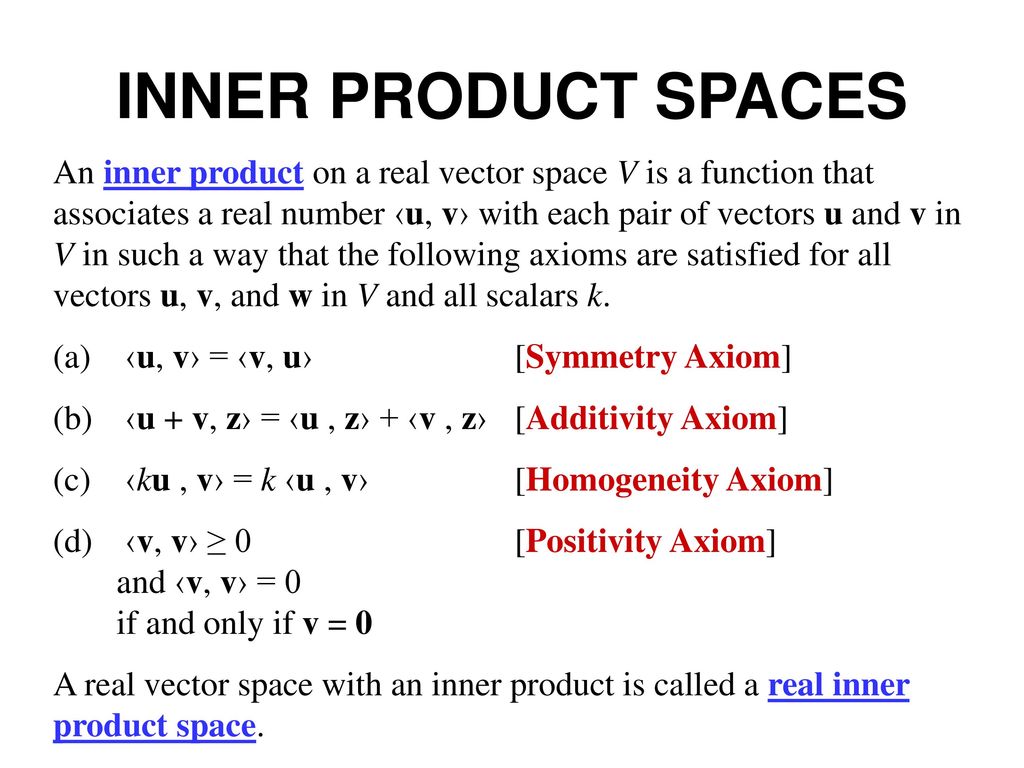
An inner product space is a vector space $V$ equipped with an inner product:

$$ \langle \vec{u}, \vec{v} \rangle $$

that returns a scalar and satisfies specific properties.

---

Inner Product Axioms

An inner product must satisfy:

---

Norm from Inner Product

The norm (length) of a vector:

$$ \|\vec{v}\| = \sqrt{\langle \vec{v}, \vec{v} \rangle} $$

---

Orthogonality in Inner Product Spaces

Vectors $\vec{u}$, $\vec{v}$ are orthogonal if:

$$ \langle \vec{u}, \vec{v} \rangle = 0 $$

---

Angle Between Vectors

$$ \cos(\theta) = \frac{\langle \vec{u}, \vec{v} \rangle}{\|\vec{u}\| \cdot \|\vec{v}\|} $$

Defines geometric notions of angle in abstract vector spaces.

---

Projection of a Vector

Projection of $\vec{u}$ onto $\vec{v}$:

$$ \text{proj}_{\vec{v}} \vec{u} = \frac{\langle \vec{u}, \vec{v} \rangle}{\langle \vec{v}, \vec{v} \rangle} \vec{v} $$

---

Inner Product Examples

Space	Inner Product Formula
$\mathbb{R}^n$	$\sum u_i v_i$
Complex vector space	$\sum u_i \overline{v_i}$
Function space (e.g. $L^2$)	$\langle f, g \rangle = \int_a^b f(x)g(x)\, dx$

---

Applications in ML & Data Science

Application	Role of Inner Product
PCA / SVD	Finding directions with high variance (via orthogonality)
Kernel methods (SVM)	Generalized inner products via kernel trick
Cosine similarity	Uses normalized inner product for text/image comparison
Orthogonalization	Gram-Schmidt in inner product spaces

---

Orthogonality and Orthonormality

Definition

• Two vectors $\vec{a}$ and $\vec{b}$ are orthogonal if:

$$ \vec{a} \cdot \vec{b} = 0 $$

This means they are perpendicular in Euclidean space.

---

Dot Product (Inner Product)

$$ \vec{a} \cdot \vec{b} = \|\vec{a}\| \|\vec{b}\| \cos(\theta) $$

• $= 0$ ⇨ $\theta = 90^\circ$, vectors are orthogonal

• For vectors in $\mathbb{R}^n$:

  $$ \vec{a} \cdot \vec{b} = \sum_{i=1}^{n} a_i b_i $$

---

Orthonormal Vectors

• Vectors are orthonormal if:

  • They are orthogonal
  • Each has unit length $\|\vec{v}\| = 1$

• Common in:

  • PCA (eigenvectors of covariance matrix)
  • SVD (columns of $U$ and $V$ are orthonormal)
  • QR decomposition

• Why it matters?

Application	Use of Orthogonality & Orthonormality
PCA	Principal components are orthogonal
Fourier Transform	Basis functions are orthonormal
Gram-Schmidt	Converts a basis into orthonormal basis
Neural Networks	Weight initialization (orthogonal init)
QR Decomposition	$A = QR$, $Q$ is orthonormal matrix
SVD	$U$ and $V$ matrices are orthonormal

---

Orthogonal Matrix

• A matrix $Q \in \mathbb{R}^{n \times n}$ is orthogonal if:

$$ Q^T Q = QQ^T = I $$

• Properties:

  • Columns (and rows) are orthonormal
  • $Q^{-1} = Q^T$
  • Preserves vector norms and angles

---

Projection onto a Vector

To project vector $\vec{a}$ onto vector $\vec{b}$:

$$ \text{proj}_{\vec{b}} \vec{a} = \frac{\vec{a} \cdot \vec{b}}{\|\vec{b}\|^2} \vec{b} $$

• The error vector $\vec{a} - \text{proj}_{\vec{b}} \vec{a}$ is orthogonal to $\vec{b}$

---

Orthogonal Complement

• The set of all vectors orthogonal to a subspace $W \subset \mathbb{R}^n$
• Denoted $W^\perp$

$$ W^\perp = \{ \vec{v} \in \mathbb{R}^n : \vec{v} \cdot \vec{w} = 0 \ \forall \vec{w} \in W \} $$

---

Gram-Schmidt Process (Orthogonalization Technique)

• Converts a set of linearly independent vectors into an orthonormal basis

Given a set of linearly independent vectors $\{ \mathbf{a}_1, \mathbf{a}_2, ..., \mathbf{a}_n \}$, we want to compute an orthonormal basis $\{ \mathbf{q}_1, \mathbf{q}_2, ..., \mathbf{q}_n \}$.

Steps: Projection → Subtraction → Normalization

1. Start with $\mathbf{u}_1 = \mathbf{a}_1$

2. For $k = 2$ to $n$:

   $$ \mathbf{u}_k = \mathbf{a}_k - \sum_{j=1}^{k-1} \text{proj}_{\mathbf{u}_j}(\mathbf{a}_k) $$

   Where projection:

   $$ \text{proj}_{\mathbf{u}_j}(\mathbf{a}_k) = \frac{\mathbf{a}_k \cdot \mathbf{u}_j}{\mathbf{u}_j \cdot \mathbf{u}_j} \mathbf{u}_j $$

3. Normalize:

   $$ \mathbf{q}_k = \frac{\mathbf{u}_k}{\|\mathbf{u}_k\|} $$

---

Example

Let’s take 2 vectors:

$$ \mathbf{a}_1 = \begin{bmatrix} 3 \\ 1 \end{bmatrix}, \quad \mathbf{a}_2 = \begin{bmatrix} 2 \\ 2 \end{bmatrix} $$

Steps: Projection → Subtraction → Normalization

Step 1:

$$ \mathbf{u}_1 = \mathbf{a}_1 = \begin{bmatrix} 3 \\ 1 \end{bmatrix} $$

Step 2:

$$ \text{proj}_{\mathbf{u}_1}(\mathbf{a}_2) = \frac{\mathbf{a}_2 \cdot \mathbf{u}_1}{\mathbf{u}_1 \cdot \mathbf{u}_1} \mathbf{u}_1 = \frac{(2)(3) + (2)(1)}{(3)^2 + (1)^2} \mathbf{u}_1 = \frac{8}{10} \mathbf{u}_1 = 0.8 \cdot \begin{bmatrix} 3 \\ 1 \end{bmatrix} = \begin{bmatrix} 2.4 \\ 0.8 \end{bmatrix} $$$$ \mathbf{u}_2 = \mathbf{a}_2 - \text{proj} = \begin{bmatrix} 2 \\ 2 \end{bmatrix} - \begin{bmatrix} 2.4 \\ 0.8 \end{bmatrix} = \begin{bmatrix} -0.4 \\ 1.2 \end{bmatrix} $$

Step 3: Normalize

$$ \mathbf{q}_1 = \frac{\mathbf{u}_1}{\|\mathbf{u}_1\|} = \frac{1}{\sqrt{10}} \begin{bmatrix} 3 \\ 1 \end{bmatrix}, \quad \mathbf{q}_2 = \frac{\mathbf{u}_2}{\|\mathbf{u}_2\|} = \frac{1}{\sqrt{1.6}} \begin{bmatrix} -0.4 \\ 1.2 \end{bmatrix} $$

Now $\mathbf{q}_1$ and $\mathbf{q}_2$ are orthonormal!

import numpy as np

def gram_schmidt(vectors):
    orthonormal_set = []
    for v in vectors:
        w = v.copy()
        for u in orthonormal_set:
            proj = np.dot(w, u) * u
            w = w - proj
        norm = np.linalg.norm(w)
        if norm == 0:
            continue
        orthonormal_set.append(w / norm)
    return np.array(orthonormal_set)

# Example
a1 = np.array([3, 1])
a2 = np.array([2, 2])
vectors = [a1, a2]

Q = gram_schmidt(vectors)
print("Orthonormal basis:")
print(Q)

Covariance and Correlation Matrices

Covariance Matrix

The covariance matrix is a square matrix that provides the covariance between pairs of variables in a dataset.

Definition:

For a dataset with $n$ variables, the covariance matrix $\Sigma$ is defined as:

$$ \Sigma = \text{cov}(\vec{X}) = \frac{1}{N-1} \sum_{i=1}^{N} (\vec{x}_i - \bar{\vec{x}})(\vec{x}_i - \bar{\vec{x}})^T $$

Where:

• $\vec{X} = \left[ \vec{x}_1, \vec{x}_2, \dots, \vec{x}_N \right]$ is the matrix of data points, each $\vec{x}_i$ is a vector of variables.
• $\bar{\vec{x}}$ is the mean vector of the data points.
• $N$ is the number of data points.

---

Covariance Between Two Variables

The covariance between two variables $X$ and $Y$ is:

$$ \text{cov}(X, Y) = \frac{1}{N-1} \sum_{i=1}^{N} (x_i - \bar{x})(y_i - \bar{y}) $$

• Positive covariance: As one variable increases, the other tends to increase.
• Negative covariance: As one variable increases, the other tends to decrease.
• Zero covariance: No linear relationship between variables.

---

Properties of Covariance Matrix

Property	Description
Symmetry	Covariance matrix is symmetric: $\Sigma = \Sigma^T$.
Diagonal elements	Represent the variance of each variable.
Off-diagonal elements	Represent the covariance between pairs of variables.
Positive semi-definiteness	Covariance matrix is always positive semi-definite.
Units	Covariance is in the units of the product of the two variables.

---

Correlation Matrix

The correlation matrix is a normalized version of the covariance matrix, where each element is divided by the product of the standard deviations of the corresponding variables.

Formula:

$$ \rho_{X,Y} = \frac{\text{cov}(X,Y)}{\sigma_X \sigma_Y} $$

Where:

• $\rho_{X,Y}$ is the correlation between variables $X$ and $Y$.
• $\sigma_X$ and $\sigma_Y$ are the standard deviations of $X$ and $Y$, respectively.

The correlation matrix $R$ is derived by normalizing the covariance matrix:

$$ R = \text{corr}(\vec{X}) = D^{-1} \Sigma D^{-1} $$

Where:

• $D$ is a diagonal matrix containing the standard deviations of each variable.

---

Properties of Correlation Matrix

Property	Description
Symmetry	Correlation matrix is symmetric: $R = R^T$.
Range	The values of the correlation coefficient range between -1 and 1:

• $\rho = 1$ means perfect positive correlation
• $\rho = -1$ means perfect negative correlation
• $\rho = 0$ means no linear correlation | | Diagonal elements | Always 1, as the correlation of a variable with itself is always 1. | | Interpretation | - Positive correlation: As one variable increases, the other tends to increase.
• Negative correlation: As one variable increases, the other tends to decrease. | | No units | Correlation is a dimensionless quantity (scaled version of covariance). |

---

Key Differences Between Covariance and Correlation Matrices

Aspect	Covariance Matrix	Correlation Matrix
Scaling	Depends on the units of the variables.	Unit-less (scaled).
Range of values	Can take any value between $-\infty$ and $\infty$.	Values range from -1 to 1.
Interpretation	Direct measure of joint variability.	Normalized measure of linear relationship.
Use	Useful for understanding the variance-covariance structure.	Useful for comparing the strength of linear relationships across different pairs.

---

Example Calculation

Given a matrix of data with 3 variables and 4 samples:

$$ X = \begin{bmatrix} 2 & 4 & 3 \\ 4 & 5 & 6 \\ 3 & 7 & 8 \\ 6 & 8 & 9 \end{bmatrix} $$

1. Step 1: Compute the mean of each column:

   • $\bar{X_1} = 3.75$
   • $\bar{X_2} = 6$
   • $\bar{X_3} = 6.5$

2. Step 2: Compute the covariance between each pair of variables.

3. Step 3: Compute the correlation matrix by dividing each covariance by the product of the corresponding standard deviations.

---

Applications

Application	Description
PCA (Principal Component Analysis)	Uses covariance matrix to find directions of maximum variance.
Portfolio Optimization	Correlation between assets is used to diversify risk.
Multivariate Analysis	Analyzing relationships and dependencies between multiple variables.
Regression Analysis	Correlation and covariance used to evaluate predictor variables.
Machine Learning	Feature selection and dimensionality reduction based on correlation.

---

import numpy as np

# Example data matrix (3 variables, 4 observations)
X = np.array([[2, 4, 3],
              [4, 5, 6],
              [3, 7, 8],
              [6, 8, 9]])

# Compute Covariance Matrix
cov_matrix = np.cov(X, rowvar=False)

# Compute Correlation Matrix
corr_matrix = np.corrcoef(X, rowvar=False)

print("Covariance Matrix:\n", cov_matrix)
print("Correlation Matrix:\n", corr_matrix)

Covariance Matrix:
 [[2.91666667 2.33333333 3.5       ]
 [2.33333333 3.33333333 4.66666667]
 [3.5        4.66666667 7.        ]]
Correlation Matrix:
 [[1.         0.74833148 0.77459667]
 [0.74833148 1.         0.96609178]
 [0.77459667 0.96609178 1.        ]]

Matrix Factorization

What Is Matrix Factorization?

Matrix factorization is the process of decomposing a matrix $A \in \mathbb{R}^{m \times n}$ into two (or more) matrices whose product approximates the original matrix.

$$ A \approx B \cdot C $$

Where:

• $A$ is the matrix to be approximated (e.g., user-item ratings matrix).
• $B$ and $C$ are factorized matrices (often lower-dimensional).

---

Common Matrix Factorization Techniques

1. Singular Value Decomposition (SVD)

   • Decomposes a matrix $A \in \mathbb{R}^{m \times n}$ into three matrices:

     $$ A = U \Sigma V^T $$

     • $U$: Left singular vectors (orthogonal)
     • $\Sigma$: Diagonal matrix of singular values
     • $V^T$: Right singular vectors (orthogonal)
   • Used in PCA and Latent Semantic Analysis (LSA).

2. Non-negative Matrix Factorization (NMF)

   • Decomposes $A$ into two matrices $W \in \mathbb{R}^{m \times k}$ and $H \in \mathbb{R}^{k \times n}$, where all elements are non-negative:

     $$ A \approx W H $$

   • Useful for text mining and image processing (e.g., topic modeling).

3. LU Decomposition

   • Factorizes a square matrix $A$ into:

     $$ A = L U $$

     • $L$: Lower triangular matrix
     • $U$: Upper triangular matrix
   • Common in solving linear systems of equations.

4. QR Decomposition

   • Decomposes $A$ into:

     $$ A = Q R $$

     • $Q$: Orthogonal matrix (columns are orthonormal)
     • $R$: Upper triangular matrix
   • Used in solving least-squares problems.

5. Cholesky Decomposition

   • For a positive-definite matrix $A$, it is decomposed into:

     $$ A = L L^T $$

     • $L$: Lower triangular matrix

---

Applications of Matrix Factorization

Use Case	Technique	Description
Recommendation Systems	SVD, NMF	Factorizes user-item interaction matrix to predict ratings
Dimensionality Reduction	SVD, PCA	Reduce dimensionality while preserving variance
Topic Modeling	NMF	Factorizes text data into topics, each represented as a combination of words
Image Compression	SVD, NMF	Decomposes image matrix to reduce storage while preserving features
Signal Processing	NMF, SVD	Decomposes signals into components for analysis or denoising
Data Compression	SVD, NMF	Reduces data size while retaining most important features

---

Key Properties of Matrix Factorization

Property	Description
Low-rank approximation	Factorization approximates matrix using fewer components
Sparsity	NMF typically enforces sparsity (non-negative elements)
Uniqueness	In general, matrix factorization does not yield a unique solution without constraints
Computational Complexity	Factorization techniques like SVD are computationally expensive (especially for large matrices)
Interpretability	Factorized matrices (especially NMF) are often easier to interpret (e.g., topics, latent features)

---

How to Perform Matrix Factorization

For SVD:

1. Compute $A = U \Sigma V^T$

2. Dimensionality reduction: Use the top $k$ singular values and vectors to approximate $A$.

   $$ A_k \approx U_k \Sigma_k V_k^T $$

For NMF:

• Objective: Find matrices $W$ and $H$ that minimize the Frobenius norm:

  $$ \| A - WH \|_F $$

  (i.e., the difference between the original matrix and the approximation).

• Use gradient descent or alternating least squares (ALS) methods for optimization.

---

🔹 Choosing the Right Factorization Method

Factorization Method	Best Use Case	Key Advantage	Limitation
SVD	Dimensionality reduction, PCA	Provides exact decomposition	Computationally expensive for large matrices
NMF	Text mining, topic modeling	Interpretability (non-negative factors)	Can only handle non-negative data
LU	Solving systems of linear equations	Fast for square matrices	Requires square matrices
QR	Solving least-squares problems	Computationally stable	Not ideal for large-scale systems

---

Example (SVD in Python)

import numpy as np

# Example matrix A
A = np.array([[1, 2, 3], [4, 5, 6], [7, 8, 9]])

# Perform Singular Value Decomposition (SVD)
U, Sigma, Vt = np.linalg.svd(A)

# Reconstruct the matrix
A_reconstructed = np.dot(U, np.dot(np.diag(Sigma), Vt))

print("Original Matrix:\n", A)
print("Reconstructed Matrix:\n", A_reconstructed)

Advanced Calculus

Functions & Graphs

• Functions & Graphs/01%3A_Functions_and_Graphs)

1️⃣ Functions Basics

• A function $f: A \to B$ maps elements from set $A$ to set $B$.
• Examples: $f(x) = x^2$, $g(x) = \sin x$, etc.
• Key properties: domain, range, injective, surjective, continuous.

---

2️⃣ Trigonometric Functions

Important identities:

• Pythagorean:

  $$ \sin^2 x + \cos^2 x = 1 $$

• Angle sum/difference:

  $$ \sin(a \pm b) = \sin a \cos b \pm \cos a \sin b $$

  $$ \cos(a \pm b) = \cos a \cos b \mp \sin a \sin b $$

• Double angle:

  $$ \sin 2x = 2 \sin x \cos x, \quad \cos 2x = \cos^2 x - \sin^2 x $$

---

3️⃣ Solving Trigonometric Equations

General steps:

• Use trig identities to simplify.
• Express equation in terms of one trig function.
• Solve for variable $x$ in the domain.

Example 1: Solve for $x$ in $\sin x = \frac{1}{2}$ on $[0, 2\pi]$

• $x = \frac{\pi}{6}$, $\frac{5\pi}{6}$

Example 2: Solve $2 \cos^2 x - 3 \sin x = 0$

• Convert using $\cos^2 x = 1 - \sin^2 x$
• Solve resulting quadratic in $\sin x$

---

4️⃣ Exponential Functions

• Form:

  $$ f(x) = a^x, \quad a > 0, a \neq 1 $$

• Properties:

  • $a^{x+y} = a^x \cdot a^y$
  • $(a^x)^y = a^{xy}$

• Natural exponential:

  $$ e^x = \lim_{n \to \infty} \left(1 + \frac{x}{n}\right)^n, \quad e \approx 2.718 $$

---

5️⃣ Logarithmic Functions

• Inverse of exponential:

  $$ y = \log_a x \iff a^y = x $$

• Properties:

  • $\log_a (xy) = \log_a x + \log_a y$
  • $\log_a \left(\frac{x}{y}\right) = \log_a x - \log_a y$
  • $\log_a (x^k) = k \log_a x$

  • Change of base formula:

    $$ \log_a x = \frac{\log_b x}{\log_b a} $$

• Common logarithms:

  • Natural log $\ln x = \log_e x$
  • Base-10 log $\log x$

---

6️⃣ Transformations of Functions

Multivariable Calculus

Limits and continuity

Derivatives

Partial Derivatives

Extrema

Integrals

Vector Calculus

• Calculus of Vector-Valued Functions/13%3A_Vector-Valued_Functions/13.02%3A_Calculus_of_Vector-Valued_Functions)
• Vector Calculus/16%3A_Vector_Calculus)

Vector Calculus Basics

---

1. Gradient (∇f)

For scalar function $f(x, y, z)$:

$$ \nabla f = \left( \frac{\partial f}{\partial x}, \frac{\partial f}{\partial y}, \frac{\partial f}{\partial z} \right) $$

• Direction of maximum increase
• Magnitude = rate of maximum increase

---

2. Divergence (∇·F)

For vector field $\vec{F} = (F_1, F_2, F_3)$:

$$ \nabla \cdot \vec{F} = \frac{\partial F_1}{\partial x} + \frac{\partial F_2}{\partial y} + \frac{\partial F_3}{\partial z} $$

• Measures outflow of a vector field (source/sink behavior)

---

3. Curl (∇×F)

$$ \nabla \times \vec{F} = \left( \frac{\partial F_3}{\partial y} - \frac{\partial F_2}{\partial z}, \frac{\partial F_1}{\partial z} - \frac{\partial F_3}{\partial x}, \frac{\partial F_2}{\partial x} - \frac{\partial F_1}{\partial y} \right) $$

• Measures rotation or circulation of a field

---

4. Laplacian (∆f or ∇²f)

For scalar function $f(x, y, z)$:

$$ \nabla^2 f = \frac{\partial^2 f}{\partial x^2} + \frac{\partial^2 f}{\partial y^2} + \frac{\partial^2 f}{\partial z^2} $$

• Used in PDEs, heat/diffusion equations

---

5. Line Integral

For scalar field $f$ over curve $C$:

$$ \int_C f \, ds $$

For vector field $\vec{F}$ over path $C$:

$$ \int_C \vec{F} \cdot d\vec{r} $$

---

6. Surface Integral

For scalar field:

$$ \iint_S f(x, y, z) \, dS $$

For vector field $\vec{F}$:

$$ \iint_S \vec{F} \cdot \vec{n} \, dS $$

---

7. Theorems (Vector Identities)

Gradient of a Constant

$$ \nabla c = 0 $$

Divergence of a Curl

$$ \nabla \cdot (\nabla \times \vec{F}) = 0 $$

Curl of a Gradient

$$ \nabla \times (\nabla f) = 0 $$

---

8. Important Theorems

Green’s Theorem (2D)

$$ \oint_C (P dx + Q dy) = \iint_R \left( \frac{\partial Q}{\partial x} - \frac{\partial P}{\partial y} \right) dxdy $$

Stokes’ Theorem (3D Curl)

$$ \oint_C \vec{F} \cdot d\vec{r} = \iint_S (\nabla \times \vec{F}) \cdot d\vec{S} $$

Divergence Theorem (Gauss)

$$ \iiint_V (\nabla \cdot \vec{F}) \, dV = \iint_S \vec{F} \cdot d\vec{S} $$

---

Jacobian and Hessian Matrices

1. Jacobian Matrix (∂f/∂x)

Used when transforming multivariate functions.

Let $\vec{f}(\vec{x}) = [f_1(x), f_2(x), ..., f_m(x)]^\top$, where $\vec{x} = [x_1, x_2, ..., x_n]^\top$

Then the Jacobian $J \in \mathbb{R}^{m \times n}$ is:

$$ J = \frac{\partial \vec{f}}{\partial \vec{x}} = \begin{bmatrix} \frac{\partial f_1}{\partial x_1} & \cdots & \frac{\partial f_1}{\partial x_n} \\ \vdots & \ddots & \vdots \\ \frac{\partial f_m}{\partial x_1} & \cdots & \frac{\partial f_m}{\partial x_n} \end{bmatrix} $$

✅ Used in:

• Chain rule (deep learning)
• Nonlinear transformations
• Backpropagation (DL)
• Jacobian determinant in volume changes (normalizing flows)

---

2. Hessian Matrix (Second Derivatives)

Used for second-order optimization analysis (e.g., Newton’s method).

Let $f: \mathbb{R}^n \to \mathbb{R}$

Then the Hessian $H \in \mathbb{R}^{n \times n}$ is:

$$ H = \nabla^2 f = \begin{bmatrix} \frac{\partial^2 f}{\partial x_1^2} & \cdots & \frac{\partial^2 f}{\partial x_1 \partial x_n} \\ \vdots & \ddots & \vdots \\ \frac{\partial^2 f}{\partial x_n \partial x_1} & \cdots & \frac{\partial^2 f}{\partial x_n^2} \end{bmatrix} $$

✅ Used in:

• Convexity check (positive semi-definite Hessian → convex function)
• Newton's method for optimization
• Taylor series expansion in multivariate calculus

---

Coordinate Systems

Optimization Techniques

Optimization algorithms are at the heart of machine learning and deep learning. They are used to minimize (or maximize) a loss (or objective) function by iteratively updating the model's parameters.

Key Concepts

• Objective Function: The objective or the loss function measures how well your model is performing. It quantifies the difference between the predicted output and the actual target.

• Goal of Optimization: Minimize the loss function.

• Variables: The following are the Parameters or the internal variables of the model that are learned during training (e.g., weights in a neural network).

• Constraints: Constraints to be met by the solution.
• Feasible Region: The subset of all potential solutions that are viable given the constraints in place.
• Gradient: It is a vector of partial derivatives of the loss function with respect to each parameter.
• The learning rate (η) controls the step size of parameter updates during optimization.
• Convex Functions: Have a single global minimum. Optimization is easier because gradient descent will always find the global minimum.
• Non-Convex Functions: Have multiple local minima. Optimization is harder because gradient descent might get stuck in a local minimum.
• Local Minima: Points where the loss function is lower than in the immediate neighborhood but not the global minimum.
• Saddle Points: Points where the gradient is zero but are neither a local minimum nor a maximum. These can slow down optimization.
• Regularization techniques prevent overfitting by adding a penalty to the loss function.
• Backpropagation is the process of computing gradients in neural networks using the chain rule of calculus.
• Epoch: One full pass through the entire training dataset.
• Iteration: One update of the model's parameters (e.g., processing one mini-batch).
• Bias: Error due to overly simplistic assumptions in the model (underfitting).
• Variance: Error due to the model's sensitivity to small fluctuations in the training set (overfitting).
• Vanishing Gradients: Gradients become very small, slowing down learning (common in deep networks).
• Exploding Gradients: Gradients become very large, causing unstable updates.
• Hyperparameters are settings that control the optimization process and model behavior. Examples:
  1. Learning rate.
  2. Batch size.
  3. Number of epochs.
  4. Momentum term.
• Convergence occurs when the optimization algorithm finds a set of parameters that minimize the loss function.
• Early stopping is a regularization technique that stops training when the validation loss stops improving, preventing overfitting.

Gradient Descent & Its Variants

Convex Functions and Optimizations